
January 19, 2023

This is the thirteenth in a series of blog posts addressing a report by Diego Escobari and Gary Hoover covering the 2019 presidential election in Bolivia. Their conclusions do not hold up to scrutiny, as we observe in our report Nickels Before Dimes. Here, we expand upon various claims and conclusions that Escobari and Hoover make in their paper. Links to posts: part one, part two, part three, part four, part five, part six, part seven, part eight, part nine, part ten, part eleven, and part twelve.
In the last post, we observed that — consistent with plausible benign explanations of the election results — relaxing the parallel trends assumption helped explain Evo Morales’s 2019 first-round victory. Even interpreting the otherwise unexplained increase in support for Morales as “fraud,” the effect is too small to be politically important. Offering the worst possible interpretation, there was fraud in the 2019 election, but it was unnecessary because Morales would have won anyway.
We also saw that Escobari and Hoover then radically reframed their analysis. They abandoned the line of inquiry where the TSE announcement “created a natural experiment.” In its place, Escobari and Hoover assumed away all benign explanations for nonparallel trends, arguing that the existence of nonparallel trends itself serves as evidence of fraud in favor of Morales.
This shift of focus reeks of post-hoc reasoning; it is utterly out of place. Indeed, Escobari and Hoover take one more bite at the apple with “difference-in-difference-in-difference” models. The idea is that if there is a double-difference in the MAS-CC vote margin, some of this could be a benign reflection of factors inducing a double-difference in the vote margin of minor parties.
There is some validity to this thinking, as voters chose Bolivia Dice No (21F) in the 2016 referendum over Movimiento Tercer Sistema (MTS) more than 4:1 in urban areas compared to less than 2:1 in rural areas. However, this is a difference-in-difference-in-difference approach in name only. The same 2016 results are used as the baseline for both the major- and minor-party double-differences. In the “triple” difference, therefore, the baselines cancel out exactly. What Escobari and Hoover actually offer is a double-difference for the major parties using the minor-party difference as a baseline. This is clear in the results of Table 1, where dropping all 2016 data from the analysis has no effect at all on the estimate.
Table 1
| Full Data | 2019 Data Only | Full Data | 2019 Data Only | |
|---|---|---|---|---|
| (1) | (2) | (3) | (4) | |
| SHUTDOWN x TREAT x Y2019 | 16.26 (0.634) | 16.26 (0.647) | ||
| SHUTDOWN x TREAT | * | 16.26 (0.634) | * | 16.26 (0.660) |
| SHUTDOWN x Y2019 | -13.26 (0.595) | -13.25 (0.607) | ||
| SHUTDOWN | 13.77 (0.624) | 0.511 (0.091) | 2.616 (0.166) | -8.018 (0.329) |
| TREAT x Y2019 | 10.95 (0.253) | 10.95 (0.258) | ||
| TREAT | * | 10.95 (0.253) | * | 10.95 (0.263) |
| Y2016 | 0.101 (0.624) | 0.090 (0.237) | ||
| Constant | -3.173 (0.238) | -3.071 (0.036) | -1.383 (0.058) | -1.707 (0.129) |
| Fixed Effects | ||||
| Precinct | Yes | Yes | ||
| Observations | 138,164 | 69,102 | 138,164 | 69,102 |
| 2 | 0.037 | 0.061 | 0.755 | 0.555 |
* Reported estimate is vanishingly small
Sources: TSE, OEP, and author’s calculations.
Table 1 shows a triple (double) difference of 16.26 percentage points, no matter whether 2016 data is included, and no matter whether geographic controls are included. Note that apart from the main results, the interpretations are not the same from one column to the next. For example, the SHUTDOWN coefficient of 13.77 in column 1 is the increase in net support for the referendum from early to late stations. In column 2, the SHUTDOWN coefficient is the increase in minor-party margins from early to late stations.
See also that the SHUTDOWN coefficient of column 2 estimates the increase in MTS-21F margin from early to late stations. This is identical to the sum of the SHUTDOWN and SHUTDOWN x Y2019 coefficients of column 1. Of course, this 0.51 percentage points plus the estimated “triple”-difference comes to 16.77 percentage points — exactly our original single-difference for MAS-CC. The results all make sense if the 2016 data simply cancels out.
We may see in Figure 1 the remaining double-differences with the minor party margins as baseline.
Figure 1
“Triple” Difference Reduces to Difference-in-Difference: With and Without Geographic Controls
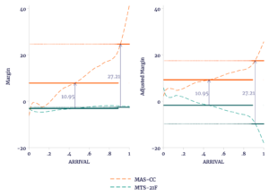
Sources: TSE, OEP, and author’s calculations.
Again, the small shares obtained by the minor parties all but demand that there can be no large trend in comparison to that of the major parties. This leaves a large double-difference of more than 16 percentage points.
Now, Escobari and Hoover claim their triple-difference comes to only 2.9 percentage points. We are completely unable to reproduce similar results and believe this is some kind of mis-specification in either theory or practice.
They write:
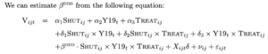
This is the full triple-difference model with some additional, largely irrelevant, controls. We may use the estimated coefficients to compute their declared result
Which is clearly not a difference-in-difference-in-difference, as this would require eight terms, consistent with the estimation model. Now, there are at least two possible explanations for this. One explanation is that Escobari and Hoover simply misreported their actual formula. Another explanation is that they mischaracterized βDDD as a triple-difference.
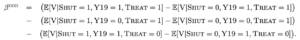
So what is βDDD if not a triple-difference? To make the notation a little more compact, we rewrite this as
Y = ([111]-[011]) – ([101]-[001]) – ([110]-[010])
A true difference-in-difference-in-difference would be
Z = ([111]-[011]) – ([101]-[001]) – ([110]-[010]) + ([100]-[000])
In Table 2, we see how to compute Yij based on the statistical model. The six terms in the formula sum not to βDDD, but to βDDD–α1
Table 2
| Cross-Station Coefficients | Station-Specific | ||||||||
|---|---|---|---|---|---|---|---|---|---|
| [111] = | 1 | 2 | 3 | 1 | 2 | 3 | +βDDD | ijδ | ij |
| -[011] = | 2 | 3 | 3 | ijδ | ij | ||||
| -[101] = | 1 | 3 | 2 | ijδ | ij | ||||
| [001] = | 3 | ijδ | ij | ||||||
| -[110] = | 1 | 2 | 1 | ijδ | ij | ||||
| [010] = | 2 | ijδ | ij | ||||||
| Y = | 1 | +βDDD |
Fortunately, this works out anyway, because SHUTDOWN is absorbed completely into the station-level effects. Escobari and Hoover do not actually estimate α1, but simply assume it to be zero.
Regardless, this triple-difference approach — reducing to a difference-in-difference between major and minor parties — to estimating fraud is even more questionable because the assumption of parallel trends is even more ephemeral. Though Escobari and Hoover again allow for nonparallel trends, they also again point to the difference in trends as indicating fraud on behalf of Morales. Even if these results could be reproduced, the interpretation is still just as faulty as it was coming from the difference-in-difference models.
Escobari and Hoover offer one more model to test for fraud: regression discontinuity. This is not the first application of regression discontinuity to the Bolivian election data. Though less formally presented, this is in effect what Irfan Nooruddin contributed to the discreditable OAS audit reports. Idrobo, Kronick, and Rodríguez address many of the shortcomings of the OAS approach in their paper. We also address conceptual problems with Nooruddin’s approach in the Annex of our previous paper.
Rather than getting into much detail, we simply observe this: to the extent that there is any meaningful discontinuity in the 2019 election data, we observe a nearly identical discontinuity in 2016. This is additional confirmation that the late 2019 results were predictable.
Figure 2
If There Is a Meaningful Discontinuity in 2019, It Persisted from 2016
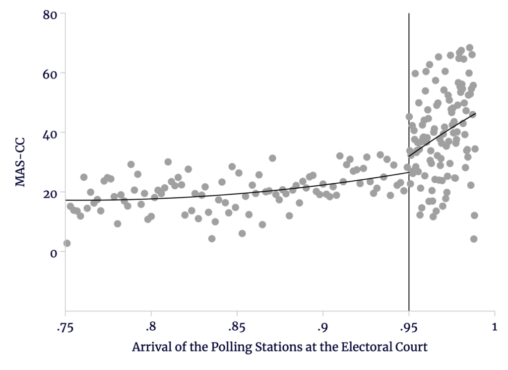
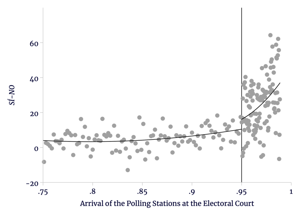
Sources: TSE, OEP, and author’s calculations.