
January 09, 2023
This is the twelfth in a series of blog posts addressing a report by Diego Escobari and Gary Hoover covering the 2019 presidential election in Bolivia. Their conclusions do not hold up to scrutiny, as we observe in our report Nickels Before Dimes. Here, we expand upon various claims and conclusions that Escobari and Hoover make in their paper. Links to posts: part one, part two, part three, part four, part five, part six, part seven, part eight, part nine,part ten, and part eleven.
In the previous post , we looked at the difference-in-difference models of Escobari and Hoover. We noted that they all show the same thing, suffering from the same problem. To identify fraud, they require that however much more the results at the late-transmitting polling stations favored Morales when contrasted with the early ones, they ought to do so by no more than the corresponding increase in the Sí vote in 2016. This is the “parallel trends” assumption. Unfortunately, even among the polling stations included in the TSE announcement, the average gap between 2016 and 2019 grows with the lateness of the transmission of results. Because the late polling stations (those excluded from the announcement) were very disproportionately late in their transmissions, we expect that the problem lies in the baseline assumption of parallel trends. Neither the addition of geographic controls nor the inclusion of a common trend improves the model in any important way. Rather, the consequence is that what Escobari and Hoover interpret as fraud in the election is almost entirely a measure of the degree to which the parallel trends assumption is wrong.
Escobari and Hoover do allow for this possibility. In their next models, they account for the linear difference in trends among the polling stations included in the announcement. Incorporating this into the model, we get Figure 1 .
Figure 1
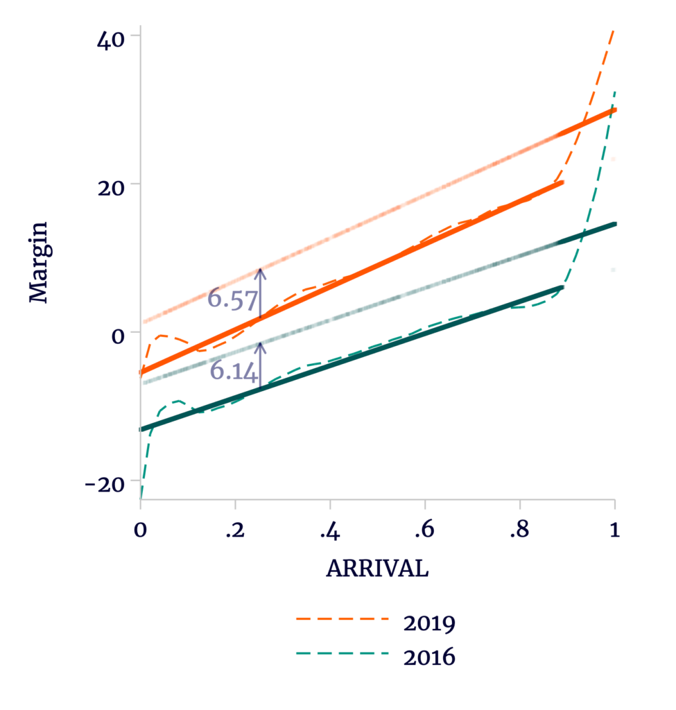
Difference-in-difference Model Allowing Different Slopes in Each Year
Sources: TSE, OEP, and author’s calculations.
For convenience, we estimate the difference-in-difference by turning the computation inside-out. In the previous post, we contrasted the difference across elections for the late-counted votes with the difference across elections for the early-counted votes. However, these differences vary with ARRIVAL. In Figure 1, we contrast the difference across late- and early-counted votes in 2019 with the difference across late- and early-counted votes in 2016. Arithmetically, this double-difference is exactly the same, but the individual differences are constant within each year.
As always, inclusion of geographic effects has no relevant impact on the estimation. We can see that in our replication, with correct valid votes and weights, that we find a much smaller double-difference: about 0.4 percentage points, compared to Escobari and Hoover’s 1 percentage point. Our estimate is not statistically significant. More importantly, none of these estimates are of political significance. Even Escobari and Hoover’s reported result leaves only 0.17 percentage points of Morales’s final margin unaccounted for.
Table 1
| As Published | Replication | Correct Voters | Weighted | |||
|---|---|---|---|---|---|---|
| (1) | (2) | (3) | (4) | (5) | (6) | |
| Variable | ||||||
| SHUTDOWN x Y2019 | 1.064 (0.390) | 0.6970 (0.409) | 0.6691 (0.408) | 0.4348 (0.277) | 0.4160 (0.288) | 0.4151 (0.391) |
| ARRIVAL x Y2019 | 5.722 (1.067) | 5.865 (0.518) | 5.876 (0.518) | 7.246 (0.345) | 7.373 (0.357) | 7.376 (0.486) |
| ARRIVAL | 21.63 (0.914) | -2.781 (0.176) | ||||
| Y2019 | * | 8.786 (0.273) | 8.792 (0.273) | 7.721 (0.180) | 7.636 (0.186) | 7.635 (0.252) |
| SHUTDOWN | 6.137 (0.691) | -0.2592 (0.128) | ||||
| Constant | * | 0.6149 (0.062) | 0.6205 (0.062) | -13.14 (0.483) | 0.5200 (0.090) | -0.9599 (0.060) |
| Fixed Effects | ||||||
| Precinct | Yes | |||||
| Station | Yes | Yes | Yes | Yes | ||
| Observations | 65,811 | 69,064 | 69,086 | 69,082 | 69,082 | 69,082 |
| R2 | 0.966 | 0.966 | 0.966 | 0.056 | 0.956 | 0.967 |
* Not reported
Sources: Escobari and Hoover, TSE, OEP, and author’s calculations.
At this point, the natural experiment is basically over. An overabundance of evidence has made it clear that parallel trends are not applicable. Even including a partial fix by allowing year-specific trends over ARRIVAL, the model successfully explains Morales’s first-round victory. Unfortunately, Escobari and Hoover then radically reframe their own experiment to argue in favor of a politically significant 2.86 percentage points of fraud in the election. They do so by shifting the focus from the double-difference to the difference in slopes, as in the right panel of Figure 2.
Figure 2
Escobari and Hoover Offer an Entirely New Interpretation of the Difference-in-Difference
Sources: TSE, OEP, and author’s calculations.
There is an obvious problem with this ex post reinterpretation of the results. Specifically, if there is fraud throughout the entire count in 2019, then we have no baseline from which to work. The TSE announcement no longer offers any opportunity to separate “untreated” (assumed fraud-free) margins from contrasting “treated” margins.
To get around this, Escobari and Hoover simply assume that only the very earliest polling stations to report are free of fraud, and reimpose the invalid parallel trends assumption. These assumptions are simply heroic.
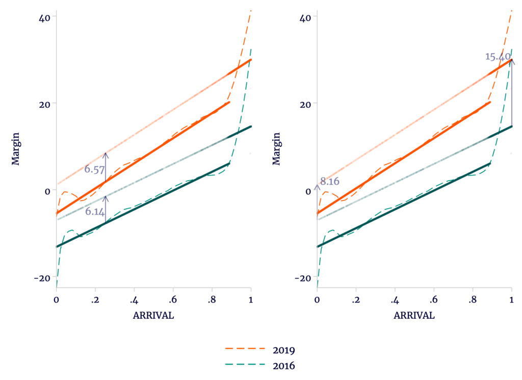
Imagine simply that Morales lost support (relative to the referendum) outside the most rural polling stations; then we might see something like Figure 3 . The gap between the opposition to the referendum (green) and support for Morales (orange) reflects Morales’s overall loss of support. Because the rural stations where Morales better held support tended to arrive late, the gap shrinks as ARRIVAL increases.
Figure 3
Different Slopes May Result from Benign Causes
Source: author’s calculations.
According to Escobari and Hoover, this cannot be an explanation for the shrinking gap. Under their assumptions, Morales could only have maintained support in rural precincts through fraud. That is, the election looks something like the left of Figure 4 , where the shaded orange area represents fraudulent votes counted for Morales in the official data. Once the shaded area is removed, the orange and green trends are made parallel.
Figure 4
Even if Trends Should Be Made Parallel, This Doesn’t Mean Fraud Favored Morales
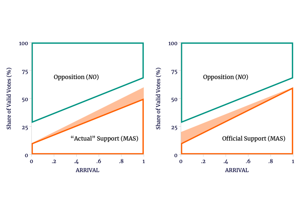
Source: author’s calculations.
However, there is an equally plausible alternative explanation: that Morales lost support in the capital cities because the opposition stole votes at these generally early polling stations where they controlled the juries. That is, we could see something like the right of Figure 4. Only after adding in the missing support for Morales are parallel trends restored. Escobari and Hoover simply assume that the left is true and the right is false.
Of course, fraud is not even necessary to explain the results at all. It could simply be true that Morales successfully maintained support in rural areas while losing ground in urban areas.
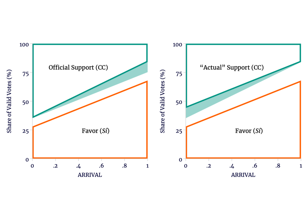
Likewise, Escobari and Hoover simply assume away the possibility that among voters opposed to the referendum Mesa’s support was disproportionately urban and in the capital cities in particular. Though we observe this in the data, Escobari and Hoover’s preferred explanation is on the left of Figure 5 : that other opposing candidates stole support for Mesa among the late arrivals. On the right, we see an alternative explanation that Mesa stole votes from other opposition candidates early.
Figure 5
The Ambiguity Persists with Different Benign Causes of the Difference in Trends
Source: author’s calculations.
Again, the only difference between the two is a presumption that the earliest results — and only the earliest results — are free of fraud.
We emphasize at this point that these two possible explanations for nonparallel trends are neither complete nor exhaustive. They are simply illustrations of benign factors that Escobari and Hoover assume away.
If we accept both of Escobari and Hoover’s incredibly strong assumptions (early arrivals being free of fraud and strict parallel trends), then there isn’t really any point in counting past the first few polling stations. Once we have the difference in margins early, we can simply compute the “fraud-free” result for the entire remainder of the election based on the 2016 results. If we complete the count, we will either find the “correct” result, or we declare fraud.
Hopefully, it is obvious that this is absurd. Escobari and Hoover’s assumptions are far too restrictive, disallowing all kinds of benign explanations of the election results. Simply put, their reinterpretation of the year-specific trends as indicating fraud is not credible.
Before we conclude this series, we will mop up the last of Escobari and Hoover’s models.