
December 06, 2022

This is the ninth in a series of blog posts addressing a report by Diego Escobari and Gary Hoover covering the 2019 presidential election in Bolivia. Their conclusions do not hold up to scrutiny, as we observe in our report Nickels Before Dimes. Here, we expand upon various claims and conclusions that Escobari and Hoover make in their paper. Links to posts: part one, part two, part three, part four, part five, part six, part seven, and part eight.
In the previous post, we adjusted the average for a precinct to match the average for the entire election while preserving the variability of polling stations within each precinct. In doing so, we eliminated the cross-precinct trend and saw that exclusion from the TSE announcement explained very little of the differences between polling stations within precincts.
The problem with this approach — as Escobari and Hoover note — is that it fails to distinguish fraud applied to an entire precinct from a precinct that for benign reasons happens to be particularly supportive of Morales. That is, while we eliminated the cross-precinct trend on the grounds that it controls for a range of benign geographic and socioeconomic explanations for the differences in support among precincts, it eliminates all illicit explanations for these precinct-level differences as well.
By way of illustration, let us add a lot (almost half a percentage point) of artificial fraud to all the polling stations that were entirely excluded from the TSE announcement. On the left of Figure 1, we see that this causes the trend to swing even more sharply upward (because these precincts tend to report late). On the right, we see that in the adjusted data there is a shift in trend among the late-transmitting polling stations (because these were disproportionately excluded from the announcement). This is the kind of “fraud” that the difference models discussed in the previous post are good at detecting.
Figure 1
Addition of Fraudulent Votes to Late Polling Stations Shows Up Despite Precinct-Level Adjustment
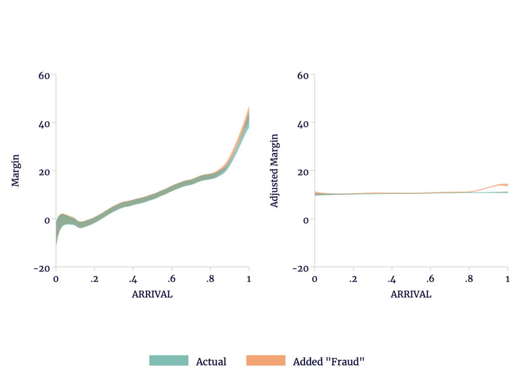
Sources: TSE and author’s calculations.
On the other hand, we can add even more fraud, but if we apply it uniformly at the precinct level among just those precincts entirely excluded from the TSE announcement, it no longer appears as a shift in the adjusted data. Instead, as we see in the right of Figure 2, it merely shifts the entire trend upward. The earlier difference models are unable to detect the addition.
Figure 2
Addition of Fraudulent Votes to Late Precincts Does Not Show Up With Precinct-Level Adjustment
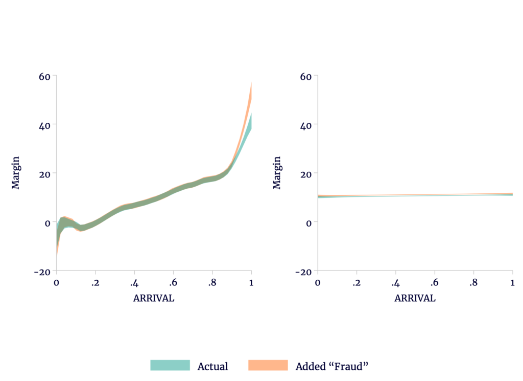
Sources: TSE and author’s calculations.
The problem is not mathematical, but conceptual. If we simply use geographic identifiers to infer differences in support for Morales among precincts, we cannot distinguish benign precinct-level differences from illicit ones. To make that distinction, we require additional information: either additional data or additional assumptions. Escobari and Hoover add both.
So what do we have? We could look for census data on population density, Internet access, Spanish fluency, educational attainment, and the like, but we are not likely to find these at a sufficiently fine geographic level to disentangle the effects. We might consider ARRIVAL itself as a control. One problem with conditioning the fraud estimate on each polling station’s position in the order of transmission is that the effect of the bias can be nonlinear over the count, even if the bias is constant. If, as we saw in post #2, the bias plausibly results in a benign, late, sharp swing in the trend, this will be difficult to disentangle from SHUTDOWN.
Escobari and Hoover chose the results of the 2016 referendum to supplement their data. As we observed in post #5, precincts with voters that more heavily favored the referendum were less fully included in the initial preliminary results announced by the TSE. In the extreme, voters at precincts entirely excluded from that announcement were on balance much more likely to support the referendum than those at precincts that were at least partially included. Support for the referendum is also a reasonable, if imperfect, proxy for political leanings. That voters supportive of the referendum might also support Morales is not surprising; approval of the referendum would have removed term limits, and Morales was the incumbent president and, at the time, was term-limited under the constitution. Geographic and socioeconomic determinants of voter behavior may affect support for both.
There are several problems with using the 2016 margins in lieu of geography. The first is it is not possible to match polling stations in 2016 to polling stations in 2019 in any simple fashion. Most obviously, the 2019 election had 34,555 tally sheets — 33,048 from within the country, and 1,507 representing voters abroad. By contrast, the 2016 vote had only 29,224 tally sheets within the country, and 1,143 abroad. There is literally no way to directly match sheets. There isn’t even a clear way to match precincts, as precinct borders moved, split, and merged between 2016 and 2019. Even precincts with the same names across different elections sometimes had different numbers of polling stations. Escobari and Hoover claim to have performed a matching of polling stations, but it is not clear how they managed it.[1]
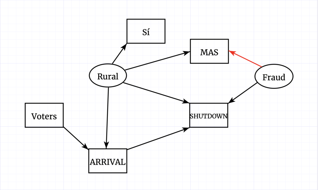
Second, the relationship between margins in 2016 and margins in 2019 is indirect, as indicated in the above diagram. By itself, a vote for the referendum in 2016 does not cause a voter to support Morales in 2019. We might guess that factors (such as socioeconomic status) that may help explain voter behavior are, over time, stable within small geographic areas such as precincts.
However, even if this is true, it doesn’t mean that the impacts of these factors on voter behavior are stable as well. The relationship between rurality and vote margin in 2016 need not be the same as the relationship between rurality and vote margin in 2019. For example, the electorate may have become more polarized, geographically, in those three years. If Morales played to a base of support in rural areas while neglecting urban areas, the change in margins across the years will vary by geography and thereby trend over the count.
There are issues with turnout as well. Turnout for the referendum was unusually low among voters residing outside Bolivia. According to a study by the OEP, reasons included nonmandatory participation, general disinterest, and seasonal travel. Those residing abroad who did turn out favored the referendum, on balance.
That aside, to the extent one might think of 2016 as a proxy for support for Morales, the relationship between the vote in 2016 and the vote in 2019 is more complex. Suppose we believe that anyone voting for the referendum would also vote for Morales. What then of those opposed to the referendum? In 2019, the opposition split among several candidates. Even if a vote for the referendum translated into a vote for Morales, it is not the case that a vote against the referendum translated into a vote for Mesa.
The split was not even stable across geographies. Mesa received 68 percent of the non-Morales valid votes in early, urban localities, compared to only 44 percent in rural localities. Mesa picked up an even larger share of the non-Morales vote in the department capitals.
| Percent of Announced Vote | Sí Share of Valid | Morales Share of Valid | Mesa Share of Non-Morales | |
|---|---|---|---|---|
| Rural | 21.47 | 65.6 | 65.3 | 45.1 |
| Foreign | 3.29 | 60.8 | 58.6 | 55.5 |
| El Alto | 10.74 | 58.5 | 55.1 | 50.8 |
| Other Urban Non-Capital | 19.37 | 49.7 | 47.5 | 60.3 |
| Capital | 45.13 | 36.4 | 32.5 | 75.9 |
| Total | 100.00 | 48.4 | 45.7 | 62.9 |
Sources: TSE and author’s calculations.
That is, from the perspective of 2016 as a proxy, Morales managed to hold ground in rural areas, though he lost a little support elsewhere. More significantly, the opposition split along geographic lines. Even within individual capital cities, Mesa picked up a lesser share of the opposition vote in precincts favoring the referendum.
Figure 3
Mesa Shares of Opposition Votes Fall With Support for Referendum (TSE Announcement)
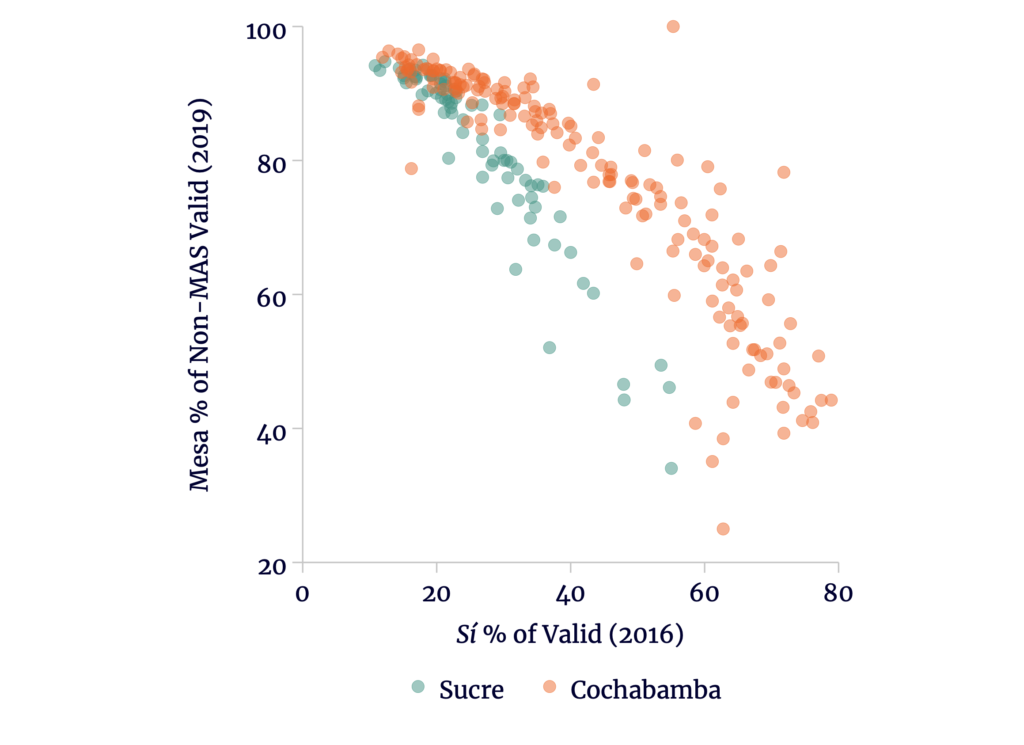
Sources: TSE and author’s calculations.
This drives a wedge between the 2016 and 2019 margins. Compared to 2016, Morales’s margin is a few percentage points better in the capital cities, but quite a bit larger in rural areas. Because of the timing differences, the trends will not be parallel. Instead, Morales’s margin will be even larger compared to the referendum among the later arrivals, and we might see something like Figure 4.
Figure 4
Margins for Morales and the Referendum at the Time of the TSE Announcement
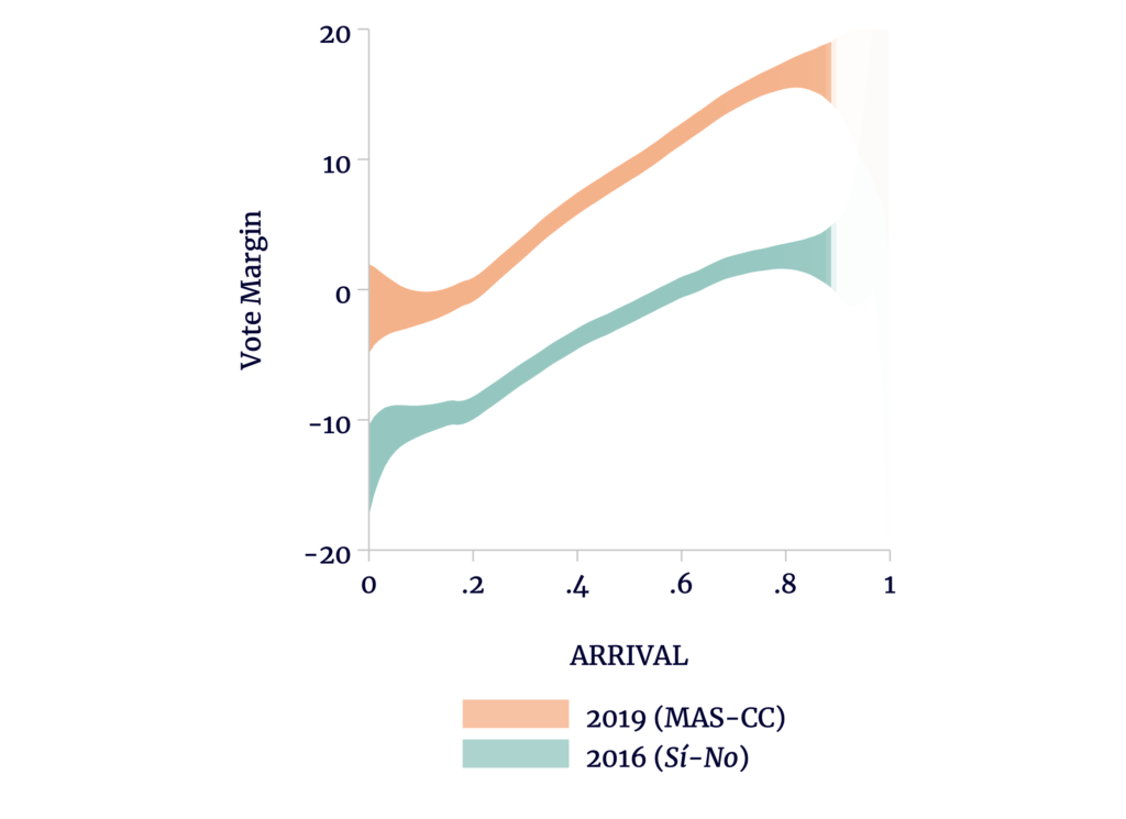
Sources: TSE, OEP, and author’s calculations.
So why does any of this matter in our understanding of Escobari and Hoover? The TSE announcement disproportionately excluded precincts where voters supported the referendum, so we expect a larger gap between 2016 and 2019 among SHUTDOWN polling stations than those included in the announcement. Yet the fundamental assumption made by Escobari and Hoover is that absent fraud, the gap should be — on average — no larger in the SHUTDOWN group. They therefore dismiss all of the above as fraud.
Regardless, Escobari and Hoover’s analyses all depend on parallel trends in fraud-free areas in order to identify fraud elsewhere. In the next post, we will see how nonparallel trends cause their models to misidentify fraud even where none exists.
Bonus Notes:
Escobari and Hoover note that “only MAS and CC appear to have experienced relatively big changes at the shutdown as the other shares of political parties in the election appear relatively stable.” In fact, as a share of the opposition vote, the CC share is one of the most stable, having fallen by 8.1 percent from 69.8 to 64.1 percent of the non-MAS valid vote. The PDC rose by 21 percent, from 16.1 to 19.5 percent; MTS by 31 percent, from 2.3 to 3.0; and MNR 27 percent, from 1.3 to 1.6. The apparent stability of the minor-party shares is precisely because they are minor parties. This will be important later on.
[1] We also performed a matching between 2016 and 2019. Our matches were sometimes approximate and were in any case at the precinct-level only. The matches we made (as well as the code to produce them) are included in the data set archived at https://github.com/ViscidKonrad/Bolivia-Escobari-Hoover.